Batch Processing of Spectra Using Sequential and Parallel Computing
This example shows how you can use a single computer, a multicore computer, or a cluster of computers to preprocess a large set of mass spectrometry signals. Note: Parallel Computing Toolbox™ and MATLAB® Parallel Server™ are required for the last part of this example.
Introduction
This example shows the required steps to set up a batch operation over a group of mass spectra contained in one or more directories. You can achieve this sequentially, or in parallel using either a multicore computer or a cluster of computers. Batch processing adapts to the single-program multiple-data (SPMD) parallel computing model, and it is best suited for Parallel Computing Toolbox™ and MATLAB® Parallel Server™.
The signals to preprocess come from protein surface-enhanced laser desorption/ionization-time of flight (SELDI-TOF) mass spectra. The data in this example are from the FDA-NCI Clinical Proteomics Program Databank. In particular, the example uses the high-resolution ovarian cancer data set that was generated using the WCX2 protein array. For a detailed description of this data set, see [1] and [2].
Setting the Repository for the Data
This example assumes that you have downloaded and uncompressed the data sets into your repository. Ideally, you should place the data sets in a network drive. If the workers all have access to the same drives on the network, they can access needed data that reside on these shared resources. This is the preferred method for sharing data, as it minimizes network traffic.
First, get the name and full path to the data repository. Two strings are defined: the path from the local computer to the repository and the path required by the cluster computers to access the same directory. Change both accordingly to your network configuration.
local_repository  = 'C:/Examples/MassSpecRepository/OvarianCD_PostQAQC/';
worker_repository = 'L:/Examples/MassSpecRepository/OvarianCD_PostQAQC/';
For this particular example, the files are stored in two subdirectories: 'Normal' and 'Cancer'. You can create lists containing the files to process using the DIR command,
cancerFiles = dir([local_repository 'Cancer/*.txt'])
normalFiles = dir([local_repository 'Normal/*.txt'])
cancerFiles =

  121×1 struct array with fields:

    name
    folder
    date
    bytes
    isdir
    datenum


normalFiles =

  95×1 struct array with fields:

    name
    folder
    date
    bytes
    isdir
    datenum
and put them into a single variable:
files = [ strcat('Cancer/',{cancerFiles.name}) ...
          strcat('Normal/',{normalFiles.name})];
N = numel(files)   % total number of files
N =

   216
Sequential Batch Processing
Before attempting to process all the files in parallel, you need to test your algorithms locally with a for loop.
Write a function with the sequential set of instructions that need to be applied to every data set. The input arguments are the path to the data (depending on how the machine that will actually do the work sees them) and the list of files to process. The output arguments are the preprocessed signals and the M/Z vector. Because the M/Z vector is the same for every spectrogram after the preprocessing, you need to store it only once. For example:
type msbatchprocessing
function [MZ,Y] = msbatchprocessing(repository,files)
% MSBATCHPROCESSING Example function for BIODISTCOMPDEMO
%
% [MZ,Y] = MSBATCHPROCESSING(REPOSITORY,FILES) Preprocesses the
% spectrogram in files FILES and returns the mass/charge (MZ) and ion
% intensities (Y) vectors.
%
% Hard-coded parameters in the preprocessing steps have been adjusted to
% deal with the high-resolution spectrograms of the example.

% Copyright 2004-2012 The MathWorks, Inc.

K = numel(files);
Y = zeros(15000,K); % need to preset the size of Y for memory performance
MZ = zeros(15000,1);

parfor k = 1:K

    file = [repository files{k}];

    % read the two-column text file with mass-charge and intensity values
    fid = fopen(file,'r');
    ftext = textscan(fid, '%f%f');
    fclose(fid);
    signal = ftext{1};
    intensity = ftext{2};

    % resample the signal to 15000 points between 2000 and 11900
    mzout = (sqrt(2000)+(0:(15000-1))'*diff(sqrt([2000,11900]))/15000).^2;
    [mz,YR] = msresample(signal,intensity,mzout);

    % align the spectrograms to two good reference peaks
    P = [3883.766 7766.166];
    YA = msalign(mz,YR,P,'WIDTH',2);

    % estimate and adjust the background
    YB = msbackadj(mz,YA,'STEP',50,'WINDOW',50);

    % reduce the noise using a nonparametric filter
    Y(:,k) = mslowess(mz,YB,'SPAN',5);

    % the mass/charge vector is the same for all spectra after the resample
    if k==1
        MZ(:,k) = mz;
    end

end
Note inside the function MSBATCHPROCESSING the intentional use of PARFOR instead of FOR. Batch processing is generally implemented by tasks that are independent between iterations. In such case, the statement FOR can indifferently be changed to PARFOR, creating a sequence of MATLAB® statements (or program) that can run seamlessly on a sequential computer, a multicore computer, or a cluster of computers, without having to modify it. In this case, the loop executes sequentially because you have not created a Parallel Pool (assuming that in the Parallel Computing Toolbox™ Preferences the checkbox for automatically creating a Parallel Pool is not checked, otherwise MATLAB will execute in parallel anyways). For the example purposes, only 20 spectrograms are preprocessed and stored in the Y matrix. You can measure the amount of time MATLAB® takes to complete the loop using the TIC and TOC commands.
tic
repository = local_repository;
K = 20; % change to N to do all

[MZ,Y] = msbatchprocessing(repository,files(1:K));

disp(sprintf('Sequential time for %d spectrograms: %f seconds',K,toc))
Sequential time for 20 spectrograms: 7.725275 seconds
Parallel Batch Processing with Multicore Computers
If you have Parallel Computing Toolbox™, you can use local workers to parallelize the loop iterations. For example, if your local machine has four-cores, you can start a Parallel Pool with four workers using the default 'local' cluster profile:
POOL = parpool('local',4);

tic
repository = local_repository;
K = 20; % change to N to do all

[MZ,Y] = msbatchprocessing(repository,files(1:K));

disp(sprintf('Parallel time with four local workers for %d spectrograms: %f seconds',K,toc))
Starting parallel pool (parpool) using the 'local' profile ...
Connected to the parallel pool (number of workers: 4).
Parallel time with four local workers for 20 spectrograms: 3.549382 seconds
Stop the local worker pool:
delete(POOL)
Parallel Batch Processing with Distributed Computing
If you have Parallel Computing Toolbox™ and MATLAB® Parallel Server™ you can also distribute the loop iterations to a larger number of computers. In this example, the cluster profile 'compbio_config_01' links to 6 workers. For information about setting up and selecting parallel configurations, see "Cluster Profiles and Computation Scaling" in the Parallel Computing Toolbox™ documentation.
Note that if you have written your own batch processing function, you should include it in the respective cluster profile by using the Cluster Profile Manager. This will ensure that MATLAB® properly transmits your new function to the workers. You access the Cluster Profile Manager using the Parallel pull-down menu on the MATLAB® desktop.
POOL = parpool('compbio_config_01',6);

tic
repository = worker_repository;
K = 20; % change to N to do all

[MZ,Y] = msbatchprocessing(repository,files(1:K));

disp(sprintf('Parallel time with 6 remote workers for %d spectrograms: %f seconds',K,toc))
Starting parallel pool (parpool) using the 'compbio_config_01' profile ...
Connected to the parallel pool (number of workers: 6).
Parallel time with 6 remote workers for 20 spectrograms: 3.541660 seconds
Stop the cluster pool:
delete(POOL)
Asynchronous Parallel Batch Processing
The execution schemes described above all operate synchronously, that is, they block the MATLAB® command line until their execution is completed. If you want to start a batch process job and get access to the command line while the computations run asynchronously (async), you can manually distribute the parallel tasks and collect the results later. This example uses the same cluster profile as before.
Create one job with one task (MSBATCHPROCESSING). The task runs on one of the workers, and its internal PARFOR loop is distributed among all the available workers in the parallel configuration. Note that if N (number of spectrograms) is much larger than the number of available workers in your parallel configuration, Parallel Computing Toolbox™ automatically balances the work load, even if you have a heterogeneous cluster.
tic % start the clock
repository = worker_repository;
K = N; % do all spectrograms
CLUSTER = parcluster('compbio_config_01');
JOB = createCommunicatingJob(CLUSTER,'NumWorkersRange',[6 6]);
TASK = createTask(JOB,@msbatchprocessing,2,{repository,files(1:K)});

submit(JOB)
When the job is submitted, your local MATLAB® prompt returns immediately. Your parallel job starts once the parallel resources become available. Meanwhile, you can monitor your parallel job by inspecting the TASK or JOB objects. Use the WAIT method to programmatically wait until your task finishes:
wait(TASK)
TASK.OutputArguments
ans =

  1×2 cell array

    {15000×1 double}    {15000×216 double}
MZ = TASK.OutputArguments{1};
Y = TASK.OutputArguments{2};
destroy(JOB) % done retrieving the results
disp(sprintf('Parallel time (asynchronous) with 6 remote workers for %d spectrograms: %f seconds',K,toc))
Parallel time (asynchronous) with 6 remote workers for 216 spectrograms: 68.368132 seconds
Postprocessing
After collecting all the data, you can use it locally. For example, you can apply group normalization:
Y = msnorm(MZ,Y,'QUANTILE',0.5,'LIMITS',[3500 11000],'MAX',50);
Create a grouping vector with the type for each spectrogram as well as indexing vectors. This "labelling" will aid to perform further analysis on the data set.
grp = [repmat({'Cancer'},size(cancerFiles));...
       repmat({'Normal'},size(normalFiles))];
cancerIdx = find(strcmp(grp,'Cancer'));
numel(cancerIdx) % number of files in the "Cancer" subdirectory
ans =

   121
normalIdx = find(strcmp(grp,'Normal'));
numel(normalIdx) % number of files in the "Normal" subdirectory
ans =

    95
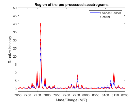
Once the data is labelled, you can display some spectrograms of each class using a different color (the first five of each group in this example).
h = plot(MZ,Y(:,cancerIdx(1:5)),'b',MZ,Y(:,normalIdx(1:5)),'r');
axis([7650 8200 -2 50])
xlabel('Mass/Charge (M/Z)');ylabel('Relative Intensity')
legend(h([1 end]),{'Ovarian Cancer','Control'})
title('Region of the pre-processed spectrograms')
Save the preprocessed data set, because it will be used in the examples Identifying Significant Features and Classifying Protein Profiles and Genetic Algorithm Search for Features in Mass Spectrometry Data.
save OvarianCancerQAQCdataset.mat Y MZ grp
Disclaimer
TIC - TOC timing is presented here as an example. The sequential and parallel execution time will vary depending on the hardware you use.
References
[1] Conrads, T P, V A Fusaro, S Ross, D Johann, V Rajapakse, B A Hitt, S M Steinberg, et al. “High-Resolution Serum Proteomic Features for Ovarian Cancer Detection.” Endocrine-Related Cancer, June 2004, 163–78.
[2] Petricoin, Emanuel F, Ali M Ardekani, Ben A Hitt, Peter J Levine, Vincent A Fusaro, Seth M Steinberg, Gordon B Mills, et al. “Use of Proteomic Patterns in Serum to Identify Ovarian Cancer.” The Lancet 359, no. 9306 (February 2002): 572–77.
See Also
msnorm | msresample | msbackadj | mslowess | msalign
You can also select a web site from the following list:
Americas
- América Latina (Español)
- Canada (English)
- United States (English)
Europe
- Belgium (English)
- Denmark (English)
- Deutschland (Deutsch)
- España (Español)
- Finland (English)
- France (Français)
- Ireland (English)
- Italia (Italiano)
- Luxembourg (English)
- Netherlands (English)
- Norway (English)
- Österreich (Deutsch)
- Portugal (English)
- Sweden (English)
- Switzerland
- United Kingdom (English)